RPACT Cloud Practical

Friedrich Pahlke

September 17, 2024

RPACT Cloud – Survival Practical

• Purpose
• Design stage
  • Required number of events
  • Required number of subjects
  • Adding an interim analysis
  • Adding a futility boundary
• Interim analysis stage with boundary re-calculation
• Final analysis stage with boundary re-calculation
• More complicated survival distributions (control arm)
• Non-proportional hazards
• Drop-outs

Purpose

We practice how to design and implement a two-arm group-sequential trial with a time-to-event endpoint, where the summary measure of interest is the hazard ratio (HR).

Design stage

Required number of events

Suppose we wish to test \(H_0 : \text{HR} \geq 1\) versus \(\text{HR} < 1\).

We require:

• One sided type 1 error probability \(\alpha = 0.025\).
• Power \(1 - \beta = 0.8\) at \(\text{HR} = 0.6\).
• Allocation ratio of 1:1.

Q1 How many events would be required for a fixed sample size design?

Required Number Of Events

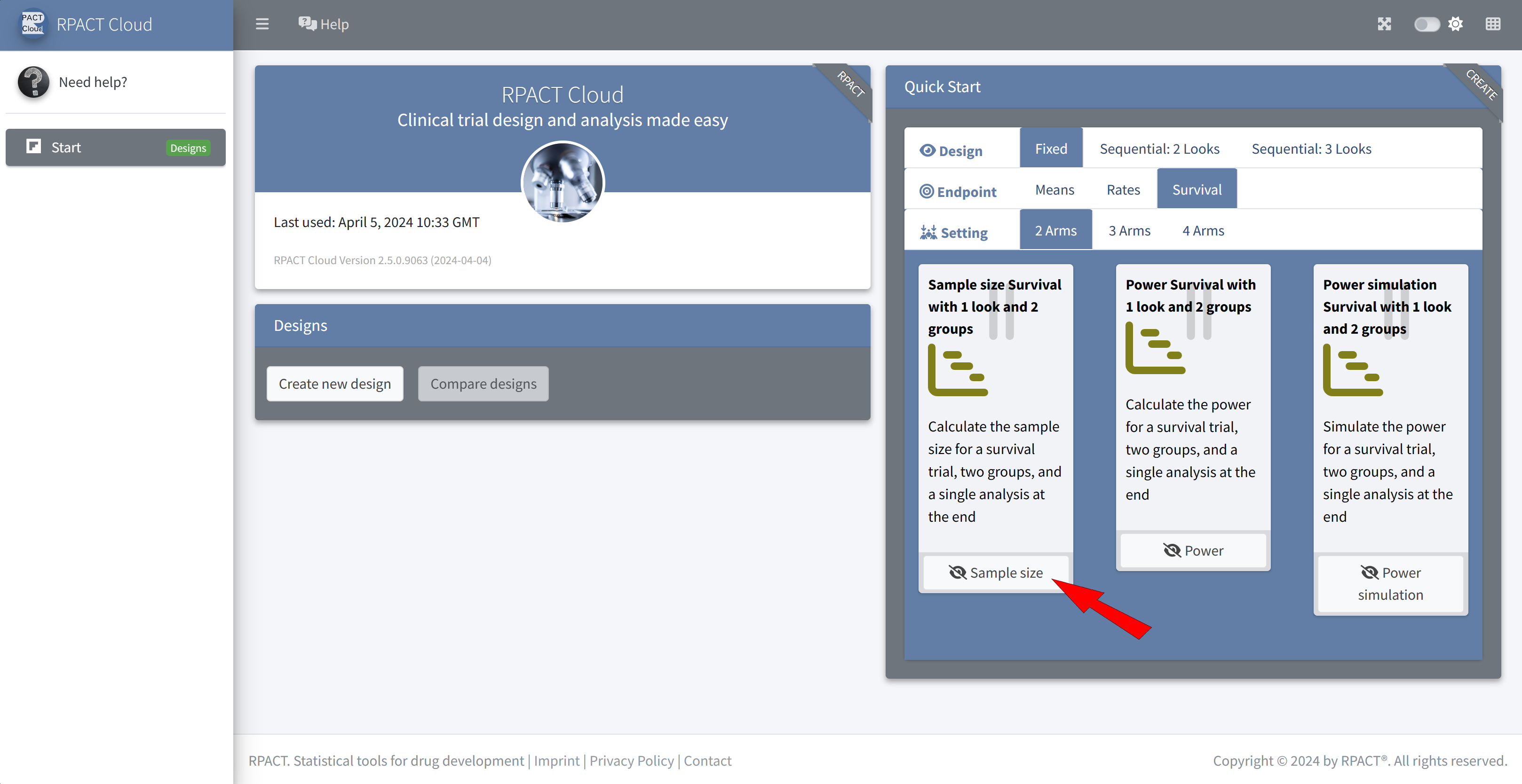
Choose Fixed, Survival, Sample size

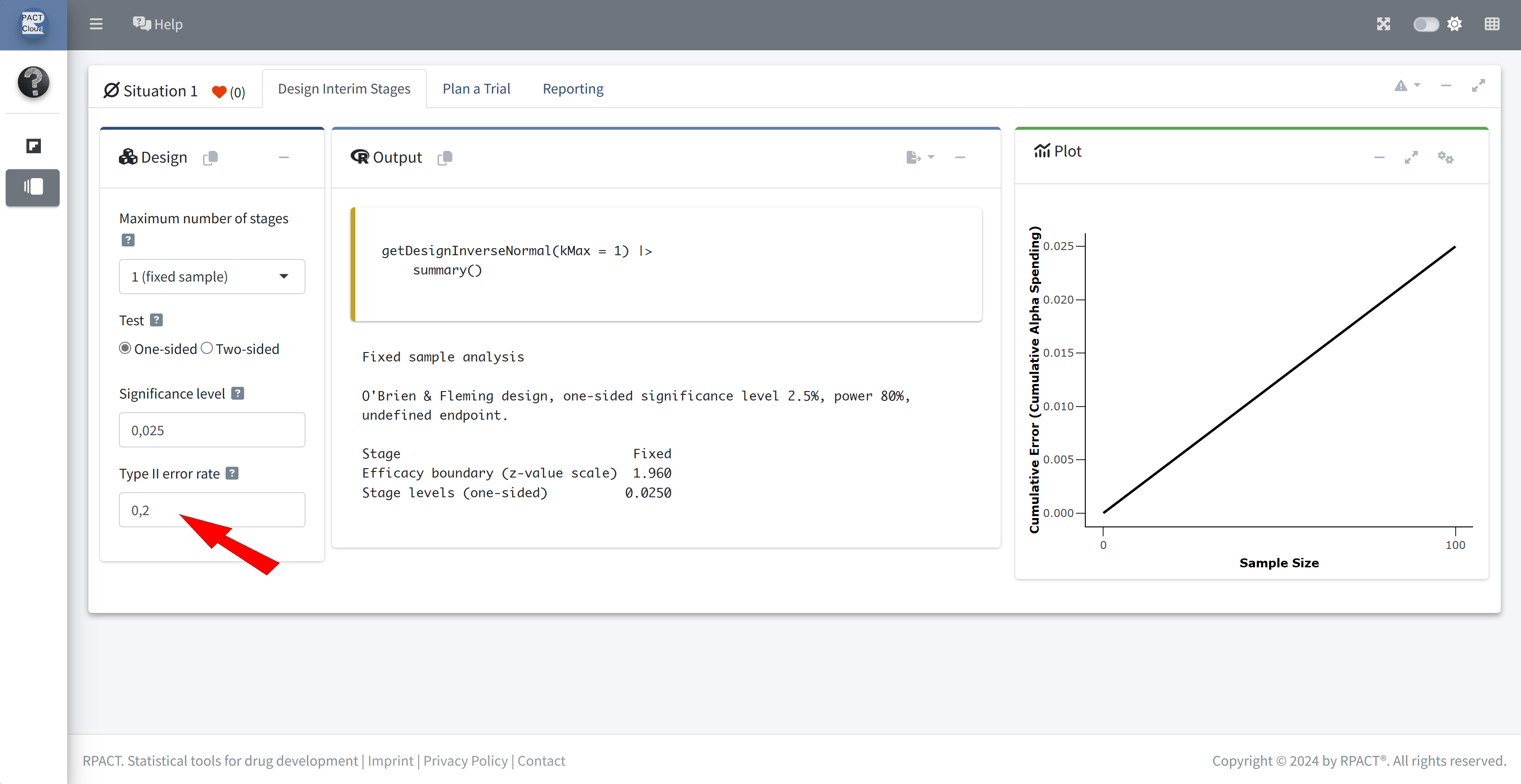
The default values of the design are identical to the example values

Go to tab “Plan a Trial”

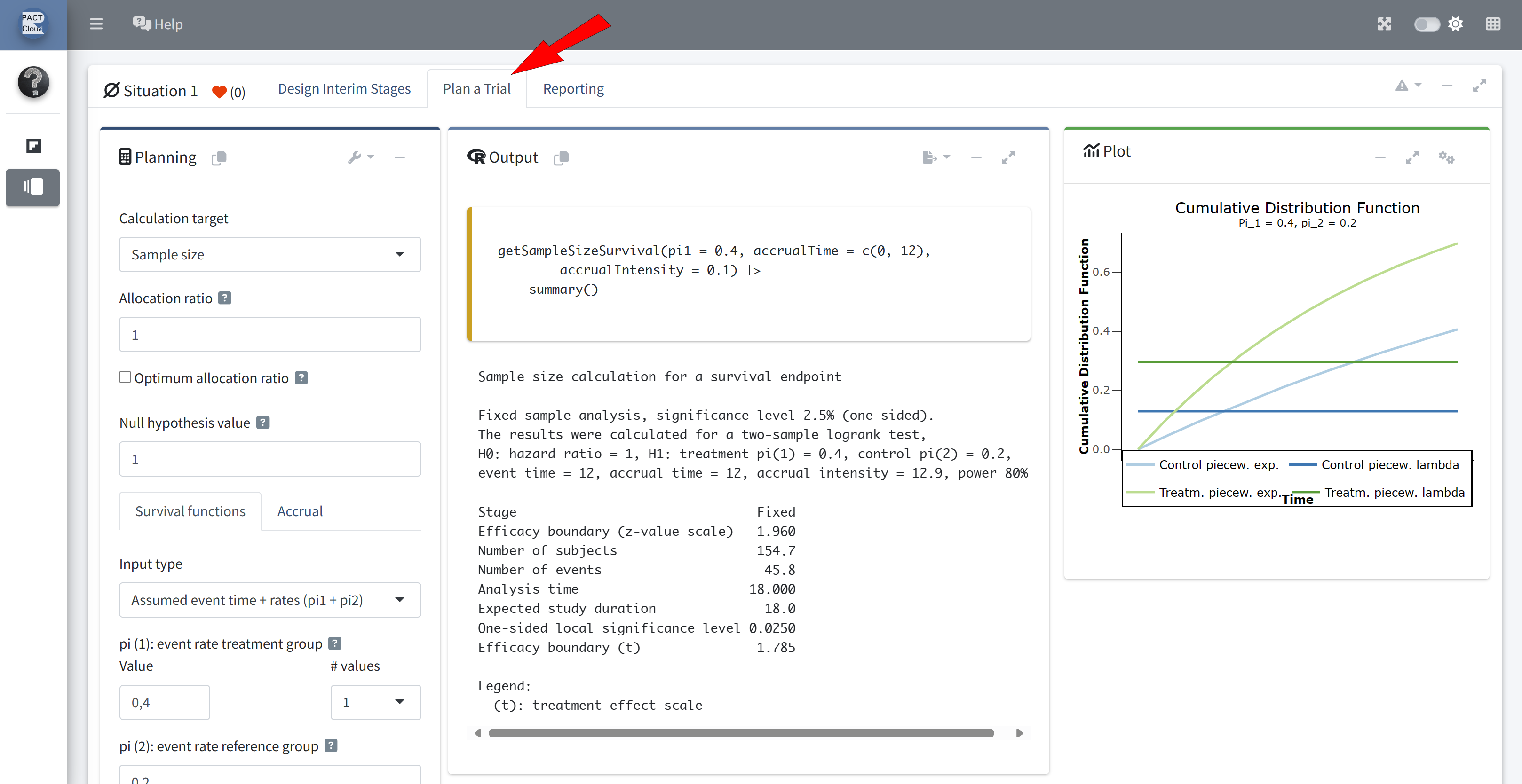
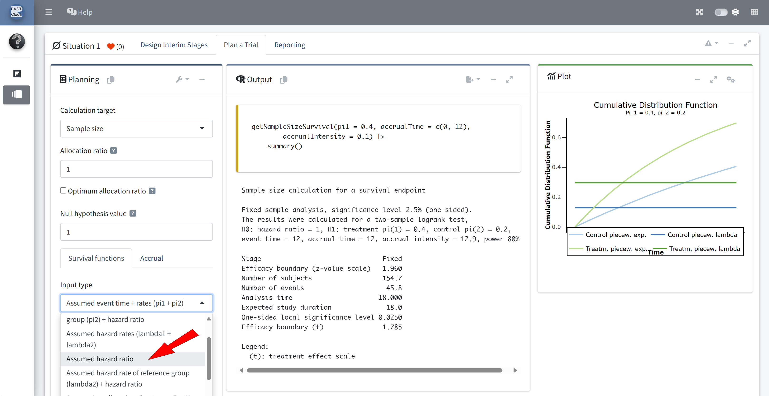
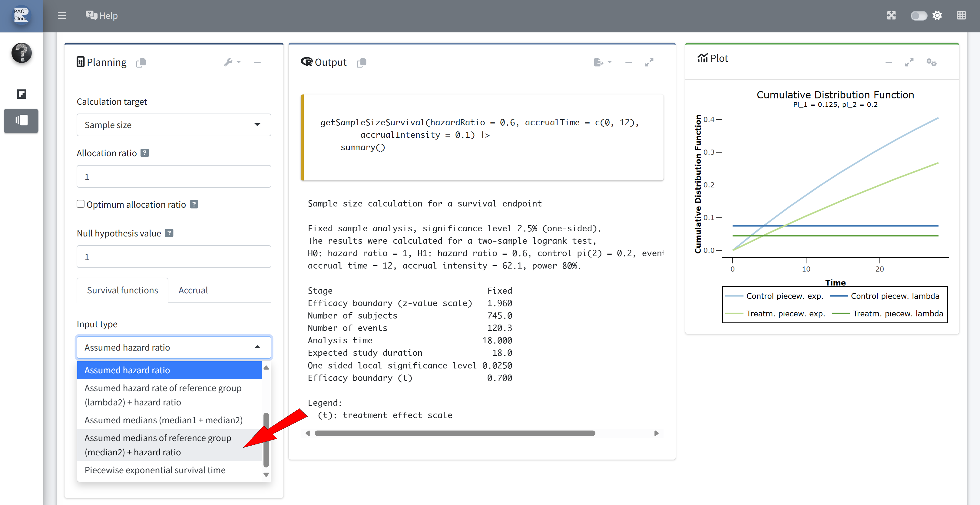
Choose an appropriate input type

Enter hazard ratio 0.6

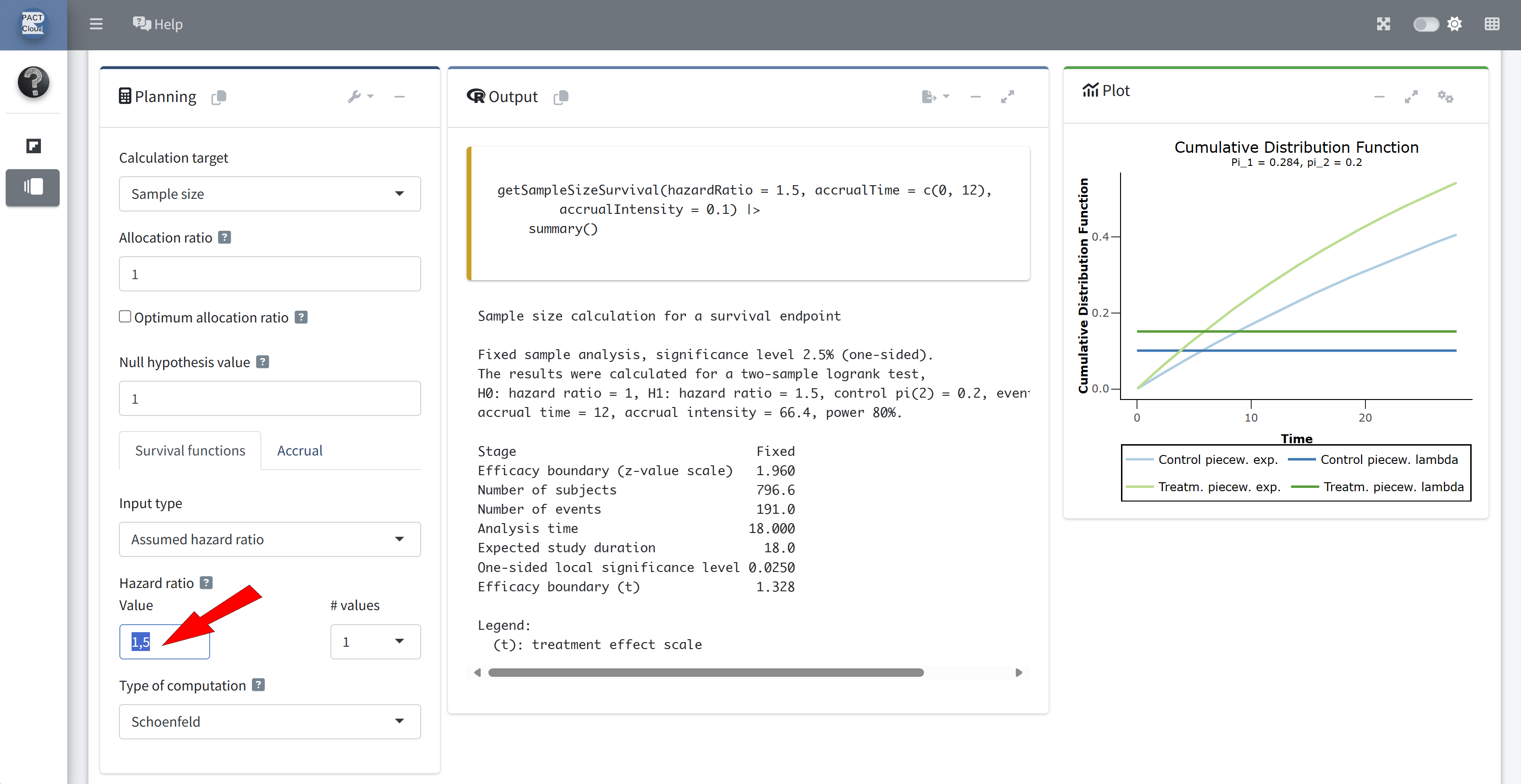
Q1 How many events would be required for a fixed sample size design? \(\rightarrow\) 121

Required Number Of Subjects

For the survival time distributions, assume:

• Median survival on the control arm is 1 year.
• Exponential distributions.

For recruitment assumptions, assume:

• It is possible to recruit 50 subjects per year at a uniform rate.
• Recruitment lasts 3 years.

Q2 What is the sample size (number of subjects) for a fixed sample size design?

Q3 What is the expected study duration for a fixed sample size design?

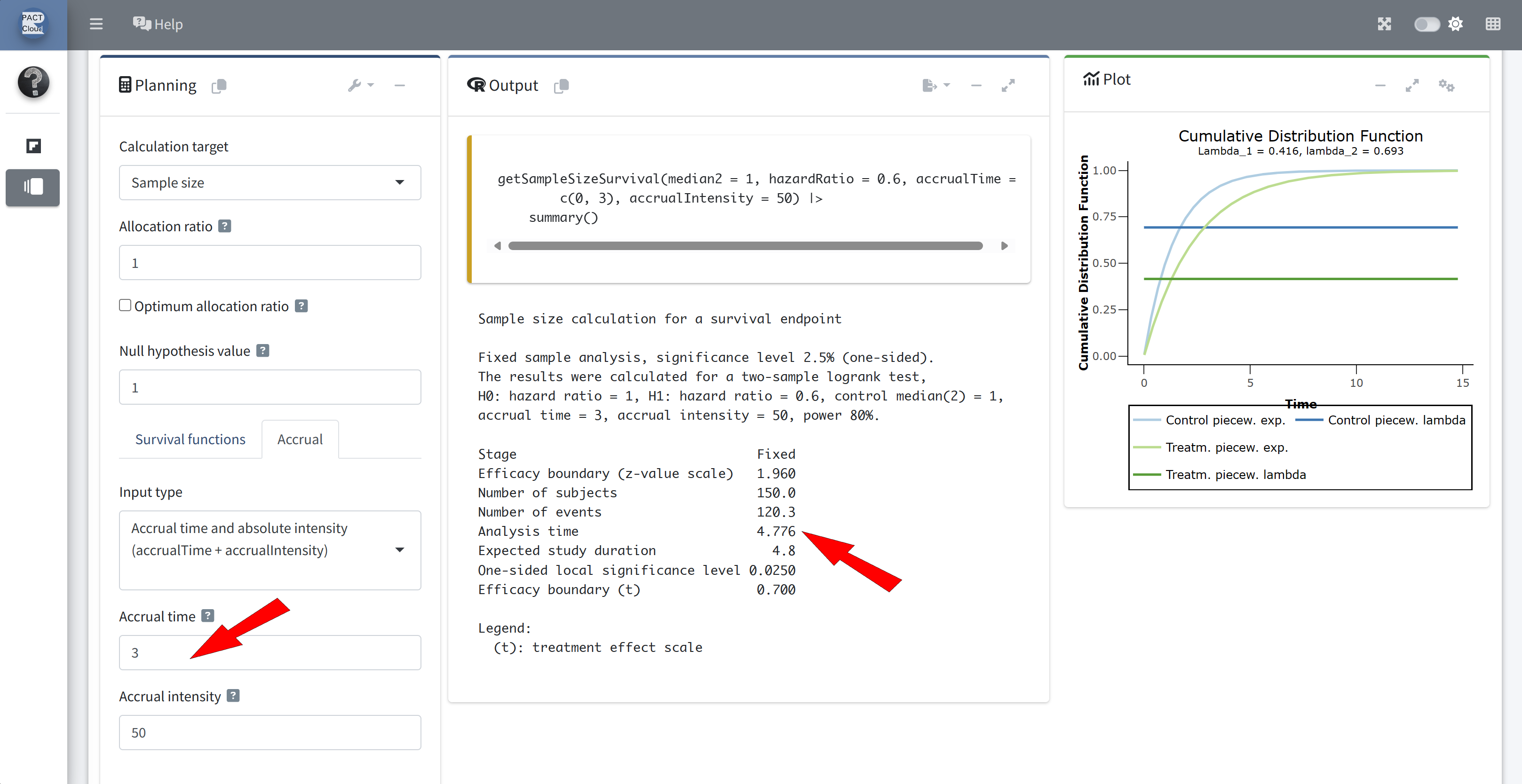
Choose an appropriate survival function input type

Enter median 1 (year)

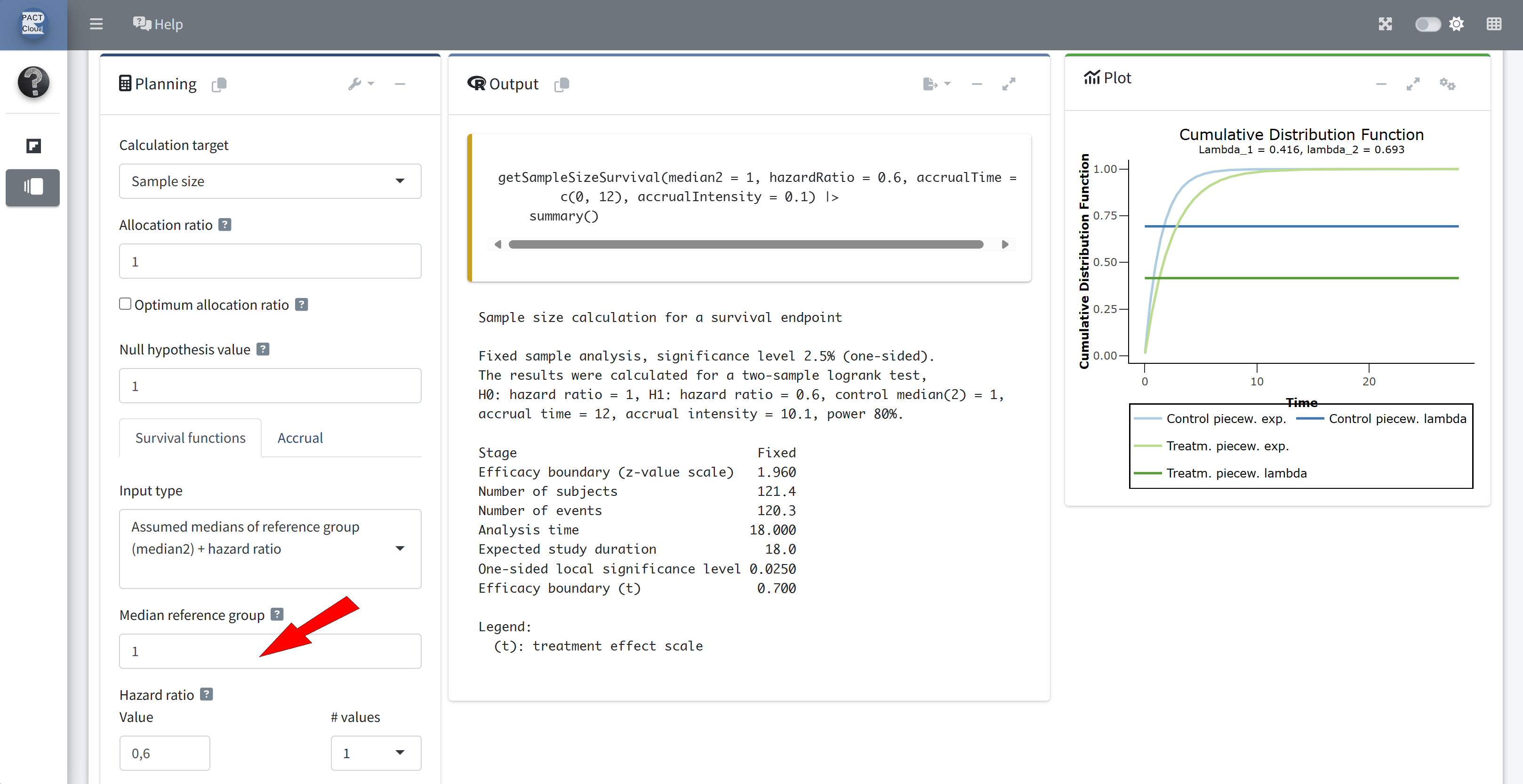
Choose an appropriate accrual time input type

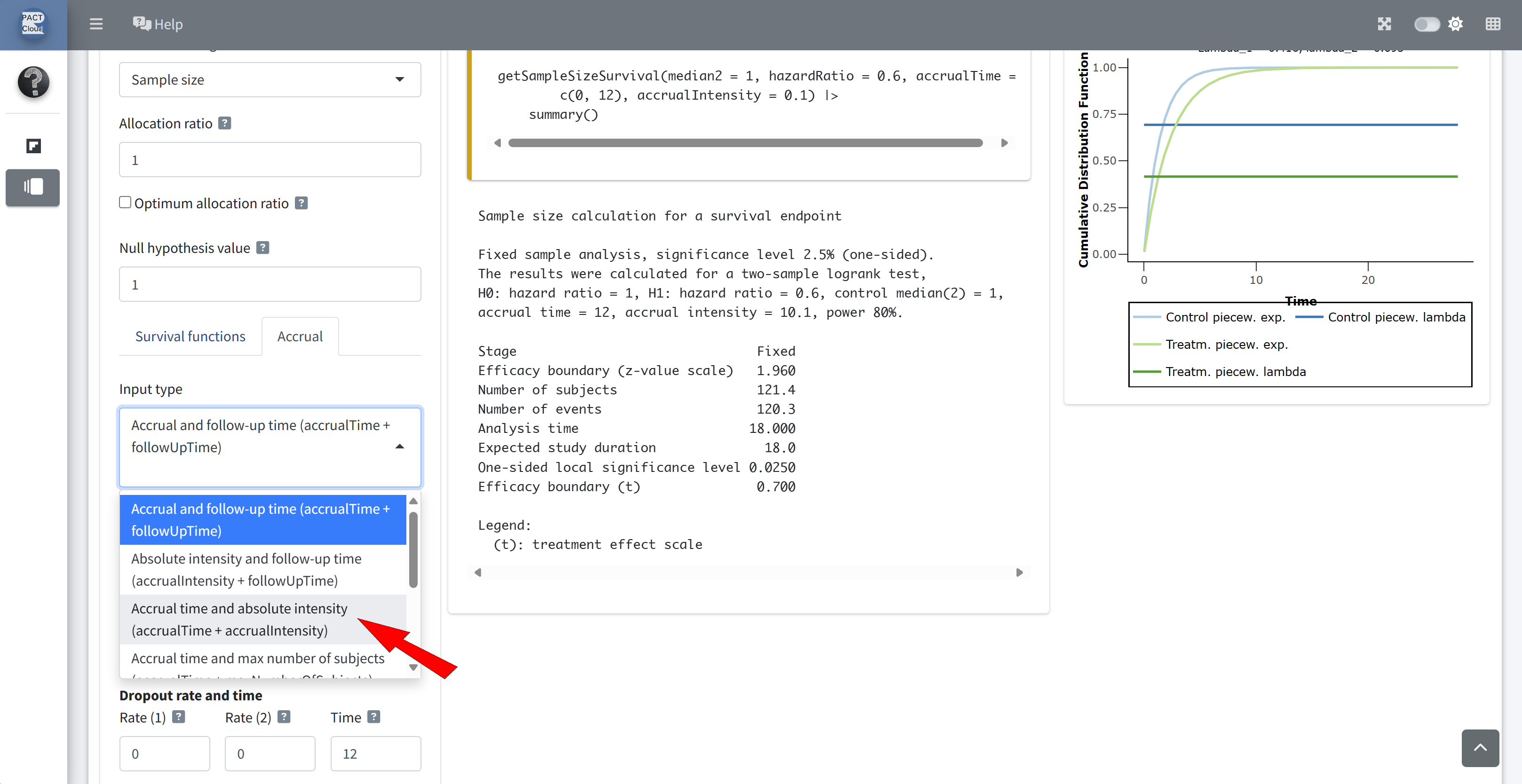
Enter accrual time 3 (years) and accrual intensity 50 \(\rightarrow\) Number of subjects = 150 (Q2)
Expected study duration (analysis time) = 4.776 years (Q3)

Q4 Suppose recruitment lasts 3.5 years instead of 3 years.
What would be the expected study duration for a fixed sample size design?

Change the accrual time to 3.5 (years) \(\rightarrow\) Expected study duration = 4.2 (years) (Q4)

Adding An Interim Analysis

• We wish to add an interim analysis for efficacy.
• The interim should happen after approximately half the required number of events.
• An O’Brien-Fleming type alpha-spending function will be used.
• No futility analysis is considered (for now).

Q5 Using the same design assumptions as above with a recruitment period of 3.5 years, prepare the sample size calculation in Q6.

Choose kMax = 2

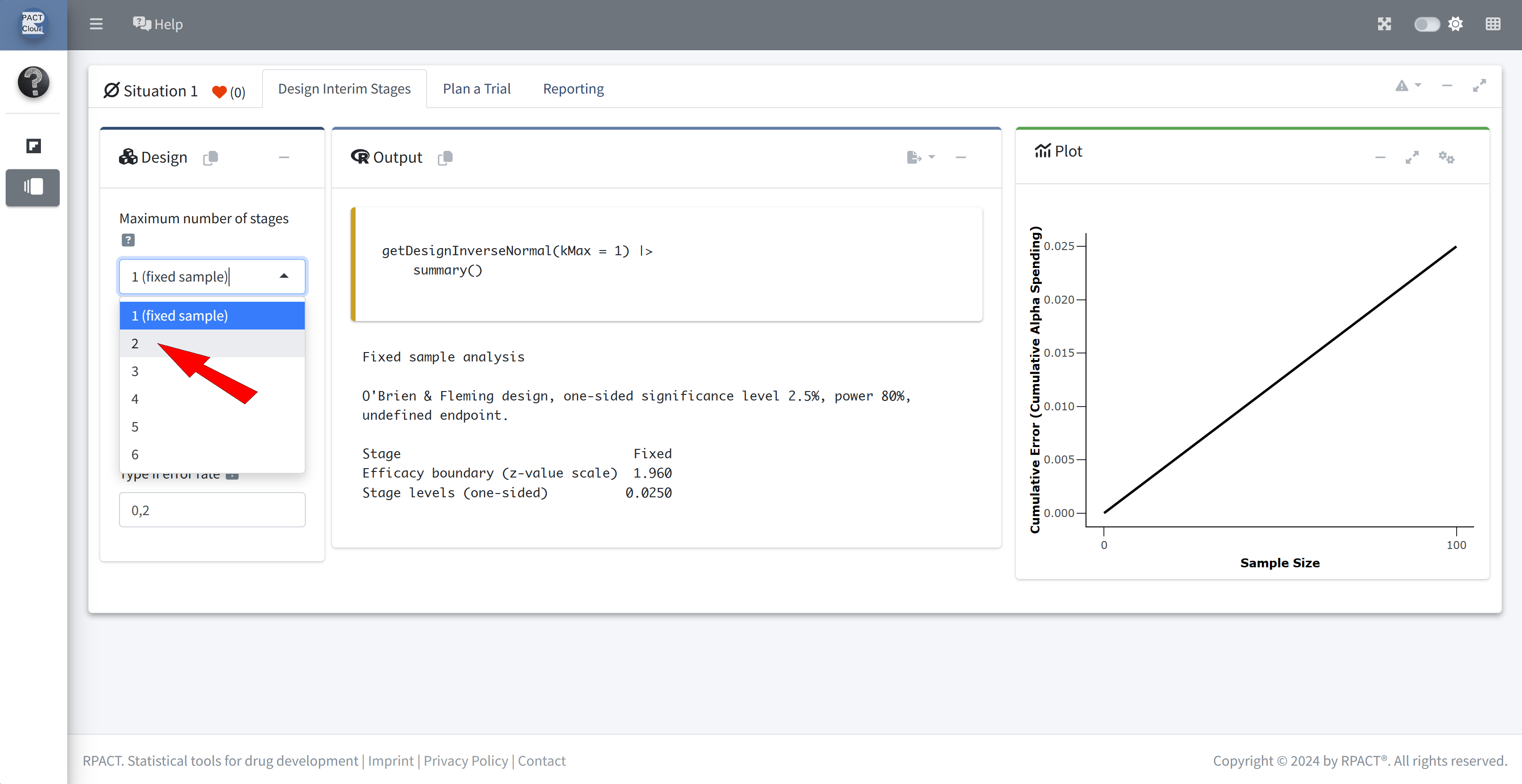
Check the information rates

Choose design type asOF

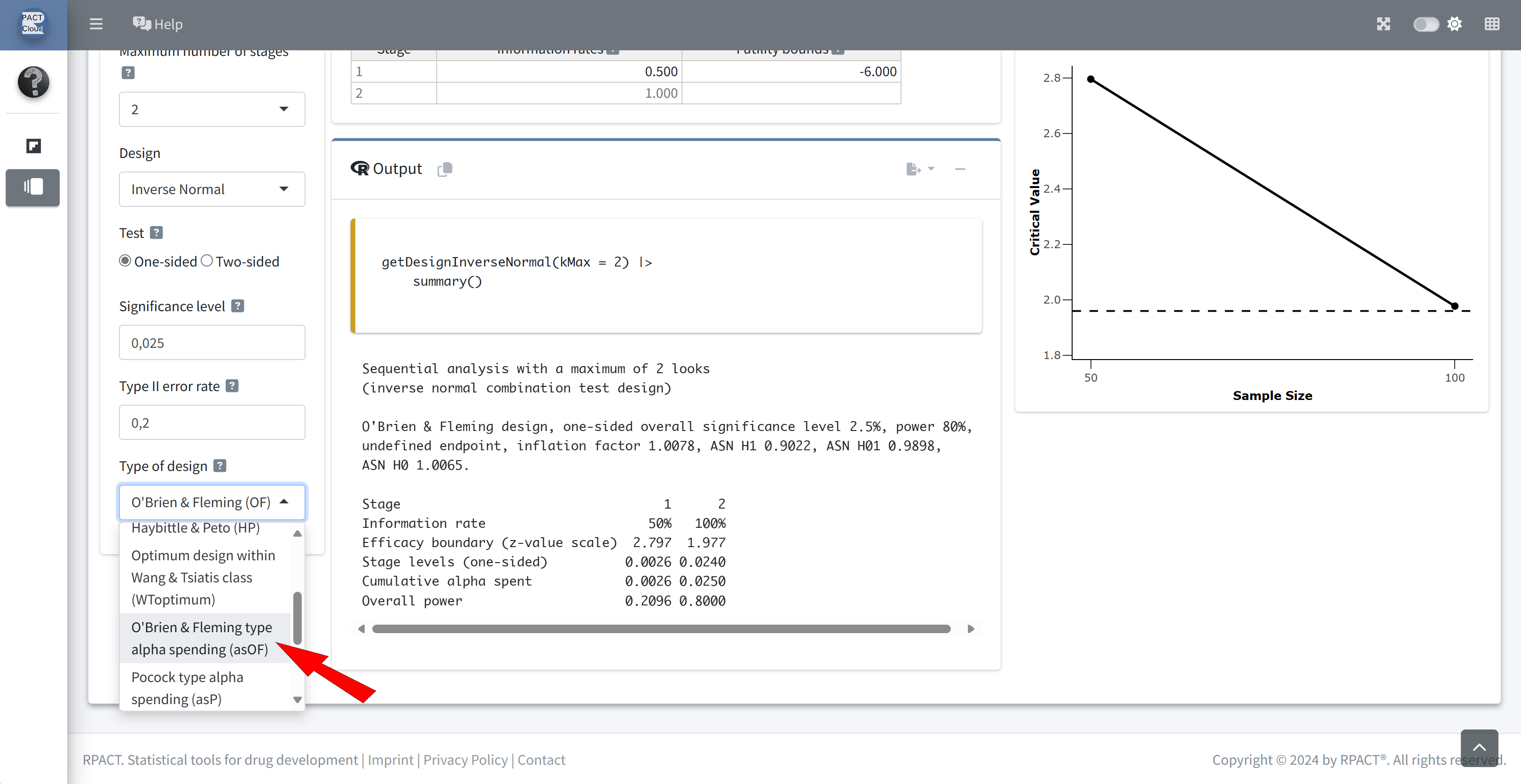
Done - Ready to perform the sample size calculation

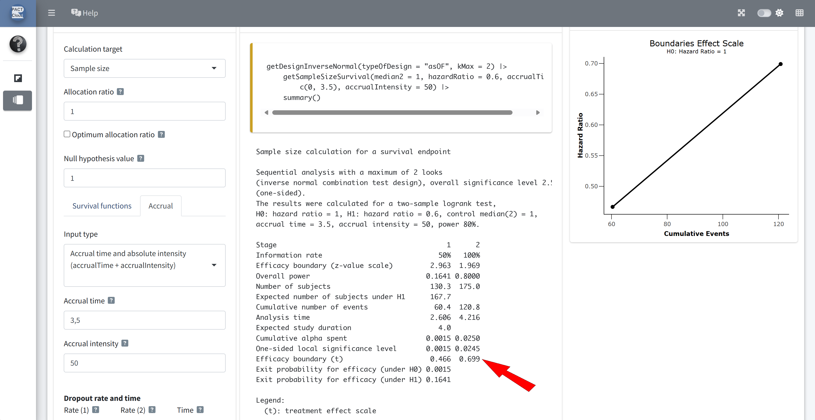
Q6 The interim analysis is planned to take place after how many events?
The final analysis is planned to take place after how many events?

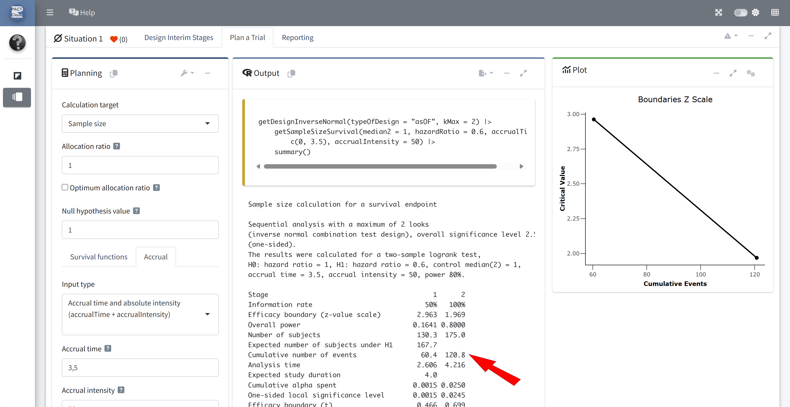
Q7 How long would it take to reach the required number of interim and final events according to the design assumptions?

Q8 What is the critical value for the hazard ratio at the interim and final analysis?

Choose output type Details instead of Summary

Q9(a) What is the expected number of events under the null hypothesis?

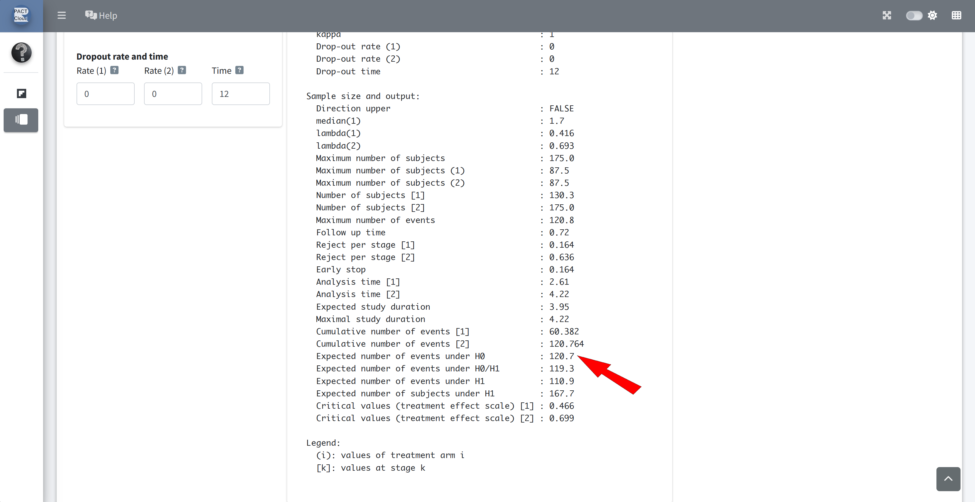
Q9(b) What is the expected number of events under the alternative?

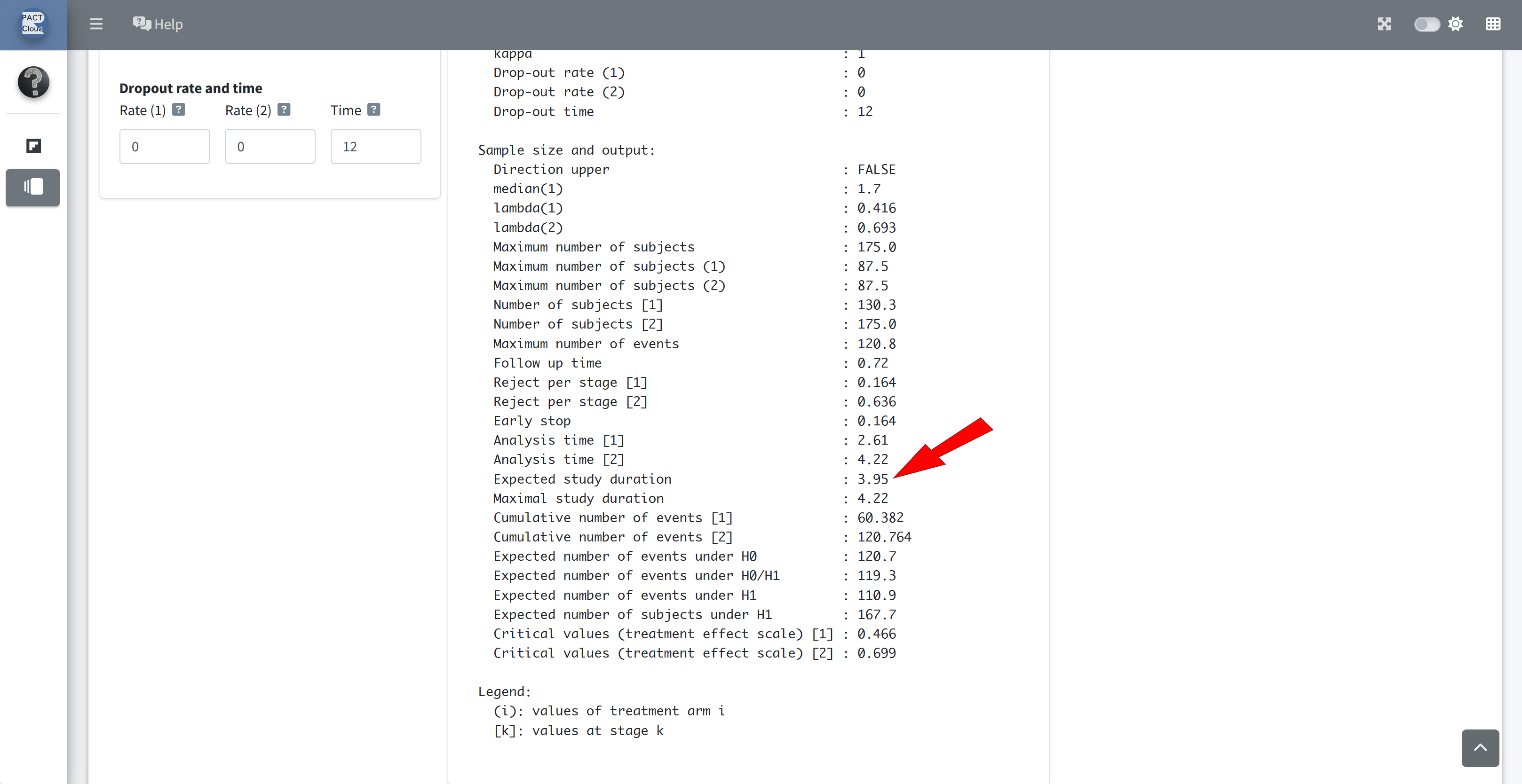
Q10 What is the expected study duration according to the design assumptions (i.e., under the alternative hypothesis)?

Q11 What is the expected number of subjects according to the design assumptions (i.e., under the alternative hypothesis)?

Adding A Futility Boundary

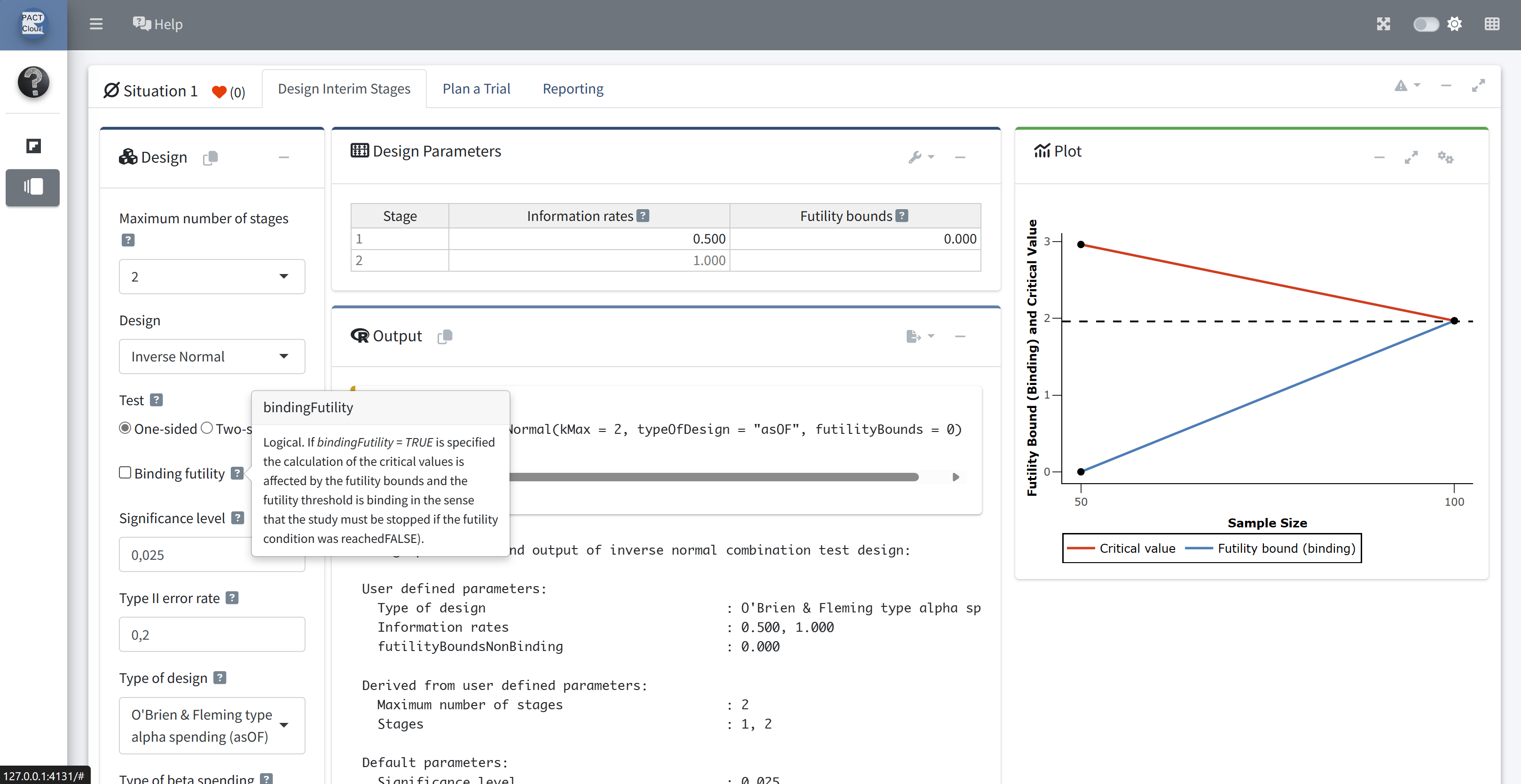
Suppose at the time of the interim analysis we wish to add a futility stopping boundary.

• A simple rule is considered.
• If the Z-statistic is above zero (where negative values of the Z-statistic indicate treatment benefit), then the trial is stopped for futility.
• However, the rule is considered non-binding.

Q12 Create a design object which includes this futility stopping rule

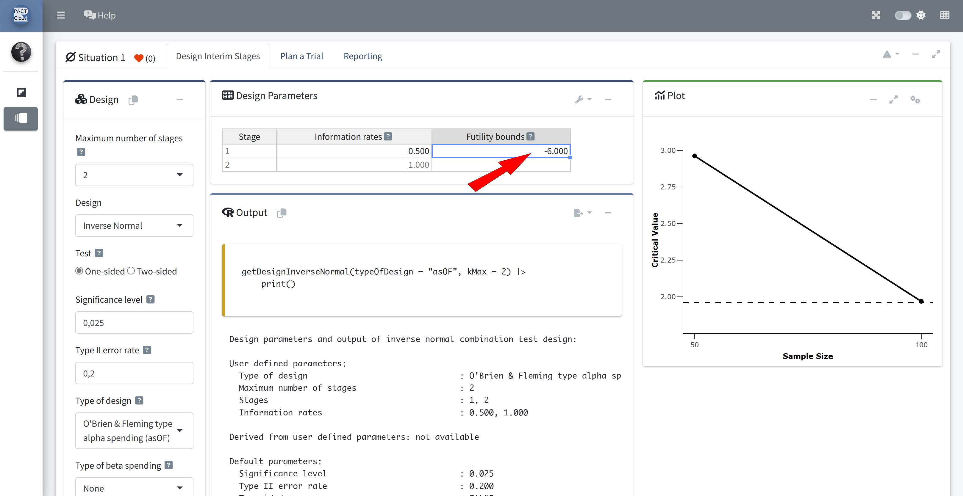
Q12 Create a design object which includes this futility stopping rule

Ensure that bindingFutility = FALSE

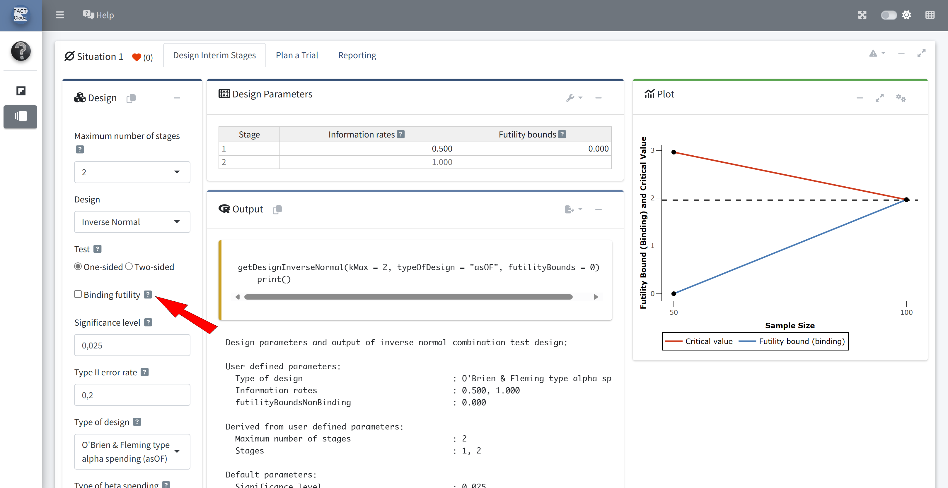
Ensure that bindingFutility = FALSE

Q13 Use the function getPowerSurvival() to calculate the overall power when adding the futility boundary under the same design assumptions as above.

• Assume recruitment lasts for 3.5 years (50 subjects per year).
• Assume that the maximum number of events is 121.

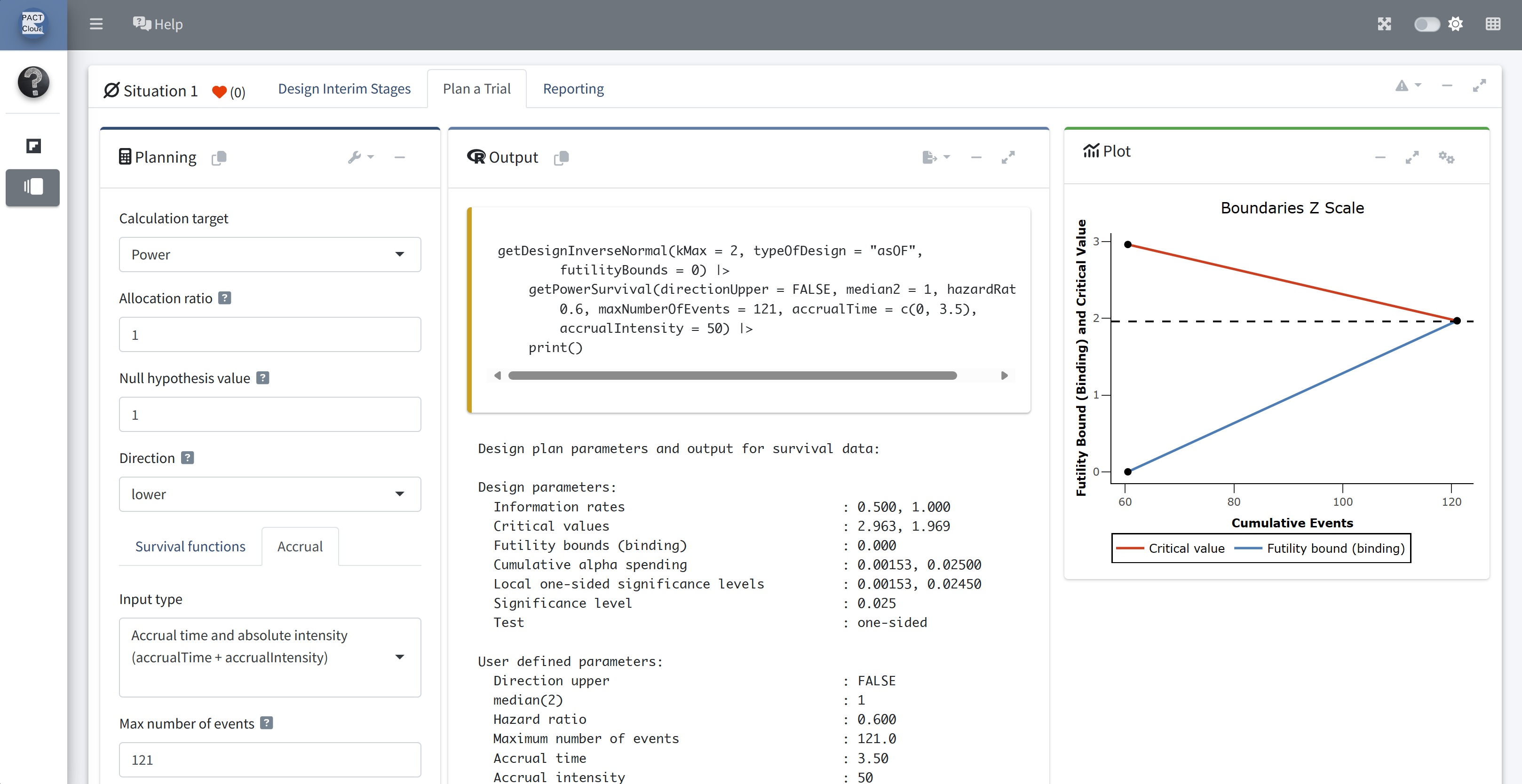
Choose calculation target “Power”

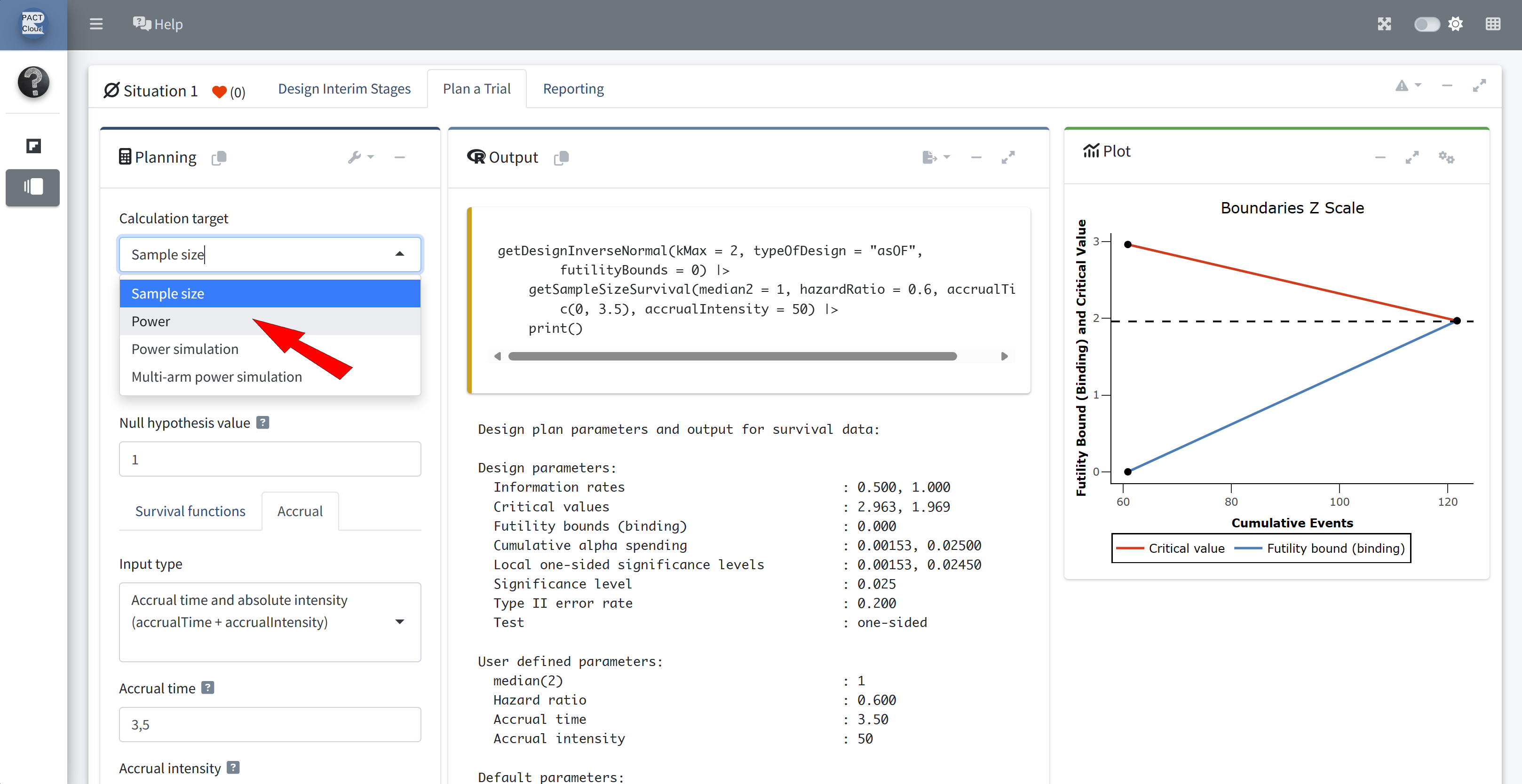
Assume: max. number of events is 121 and recruitment lasts for 3.5 years (50 subjects per year)

Set the direction to lower (directionUpper = FALSE)

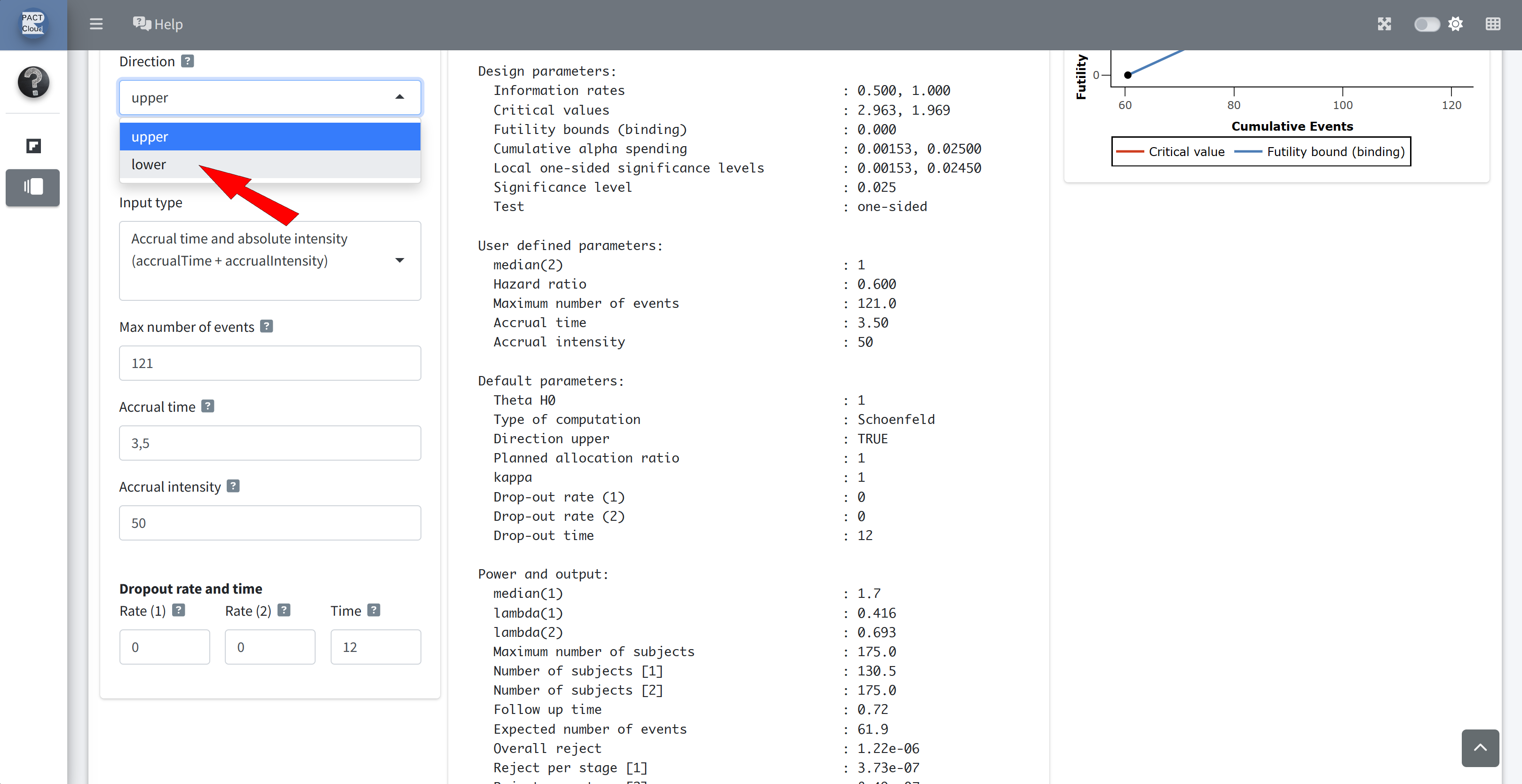
Scroll down to see the results

Q13 What is the the overall power? Q14 The expected study duration and number of subjects?

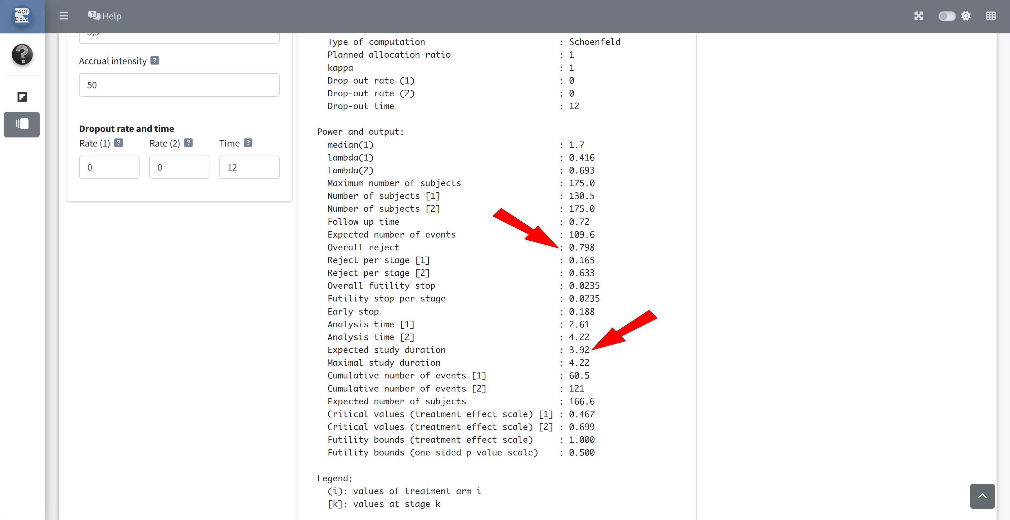
Q15 What is the expected study duration and number of subjects, under H0? Set HR to 1

Q15 What is the expected study duration and number of subjects, under the null hypothesis?

Interim Analysis Stage with Boundary Re-Calculation

Suppose at the interim analysis, the observed number of events is 67 and the value of the Z-statistic is -1.10 (where negative values correspond to treatment benefit).

Q16 Re-calculate the stopping boundary based on the observed 67 events at the interim analysis.

• Assume the same alpha-spending function as above.
• Assume the planned maximum number of events is 121.

Note

See the vignette An Example to Illustrate Boundary Re-Calculations during the Trial with rpact for background information and a description of the general principles for boundary re-calculations.

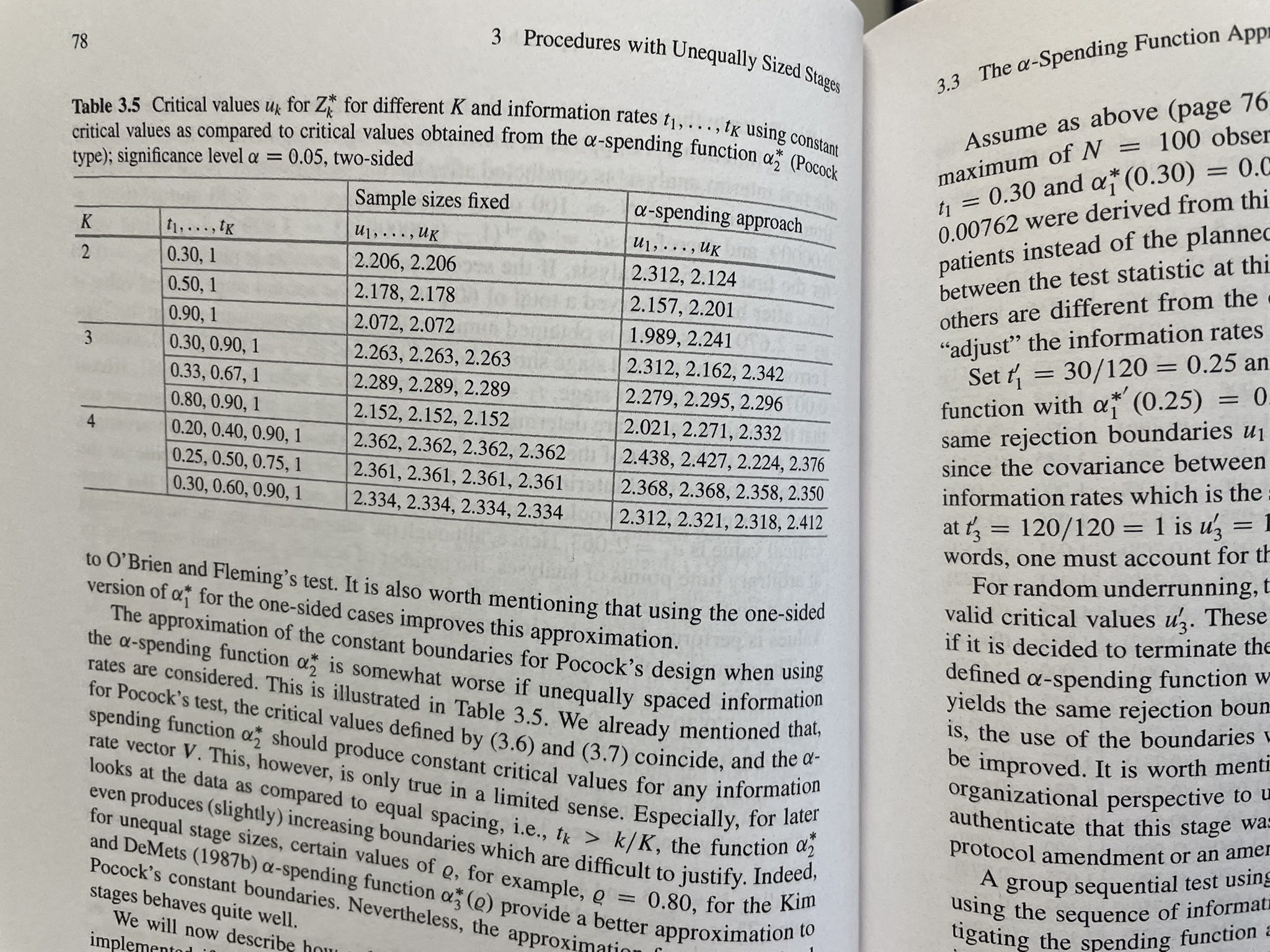
See also, Wassmer & Brannath, 2016, p78f

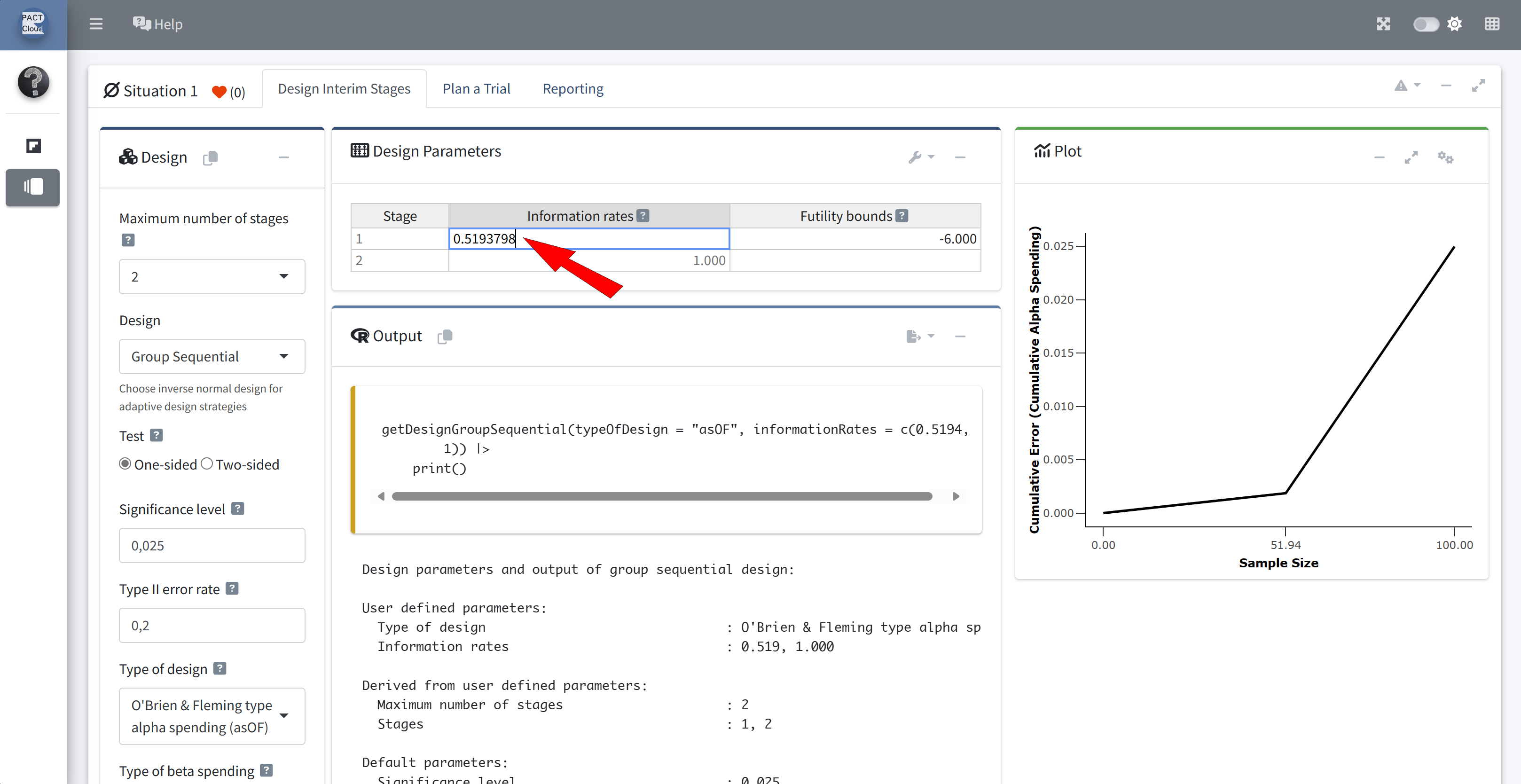
Choose group sequential design

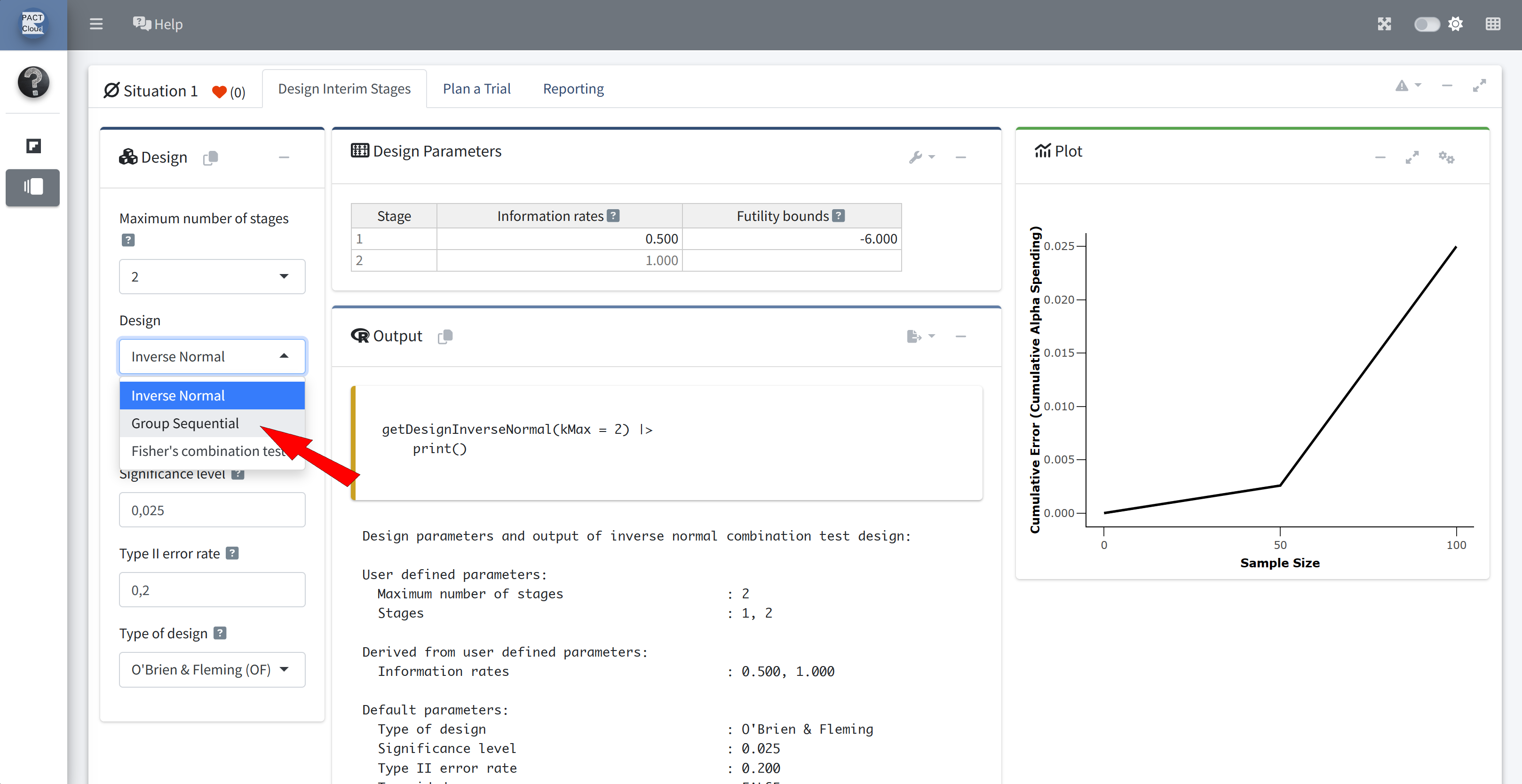
informationRates = c(67/121, 1)

Check the critical values: the stopping boundary at stage 1 is 2.795 (Q16)

Remember how much alpha was actually spent at interim: 0.00259 (required at final analysis)

Q17 What is the interim analysis decision?

Continue to the next stage, since the Z statistic -1.10 is between 0 (futility bound) and -2.795 (efficacy bound)

Note

In the current rpact version 4.0.0 the function getDesignGroupSequential() doesn’t know which direction of Z statistic indicates treatment benefit. By default, the critical values are displayed assuming positive Z is beneficial. Only when using functions like getSampleSizeSurvival() or getPowerSurvival() do we indicate the direction.

Final Analysis Stage with Boundary Re-Calculation

Suppose at the final analysis, the observed number of events is 129 and the value of the Z-statistic is -2.00 (where negative values correspond to treatment benefit).

Q18 Re-calculate the stopping boundary based on the observed 67 events at interim and 129 events at the final analysis.

Note

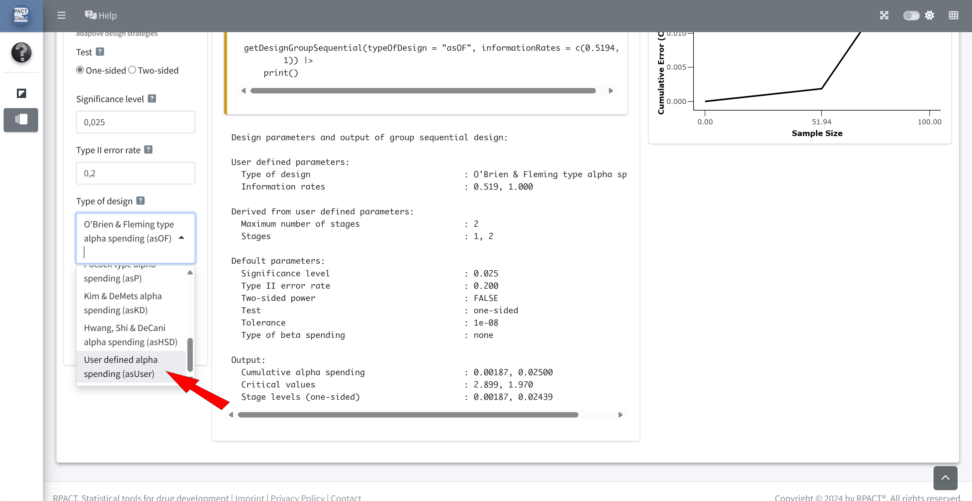
Since we have deviated from the planned number of events, our actual alpha spent no longer follows the O’Brien-Fleming-type alpha-spending function. Use the argument typeOfDesign = "asUser" instead.

Note

Since the observed information at the final analysis (129) is larger than the planned maximum information (121) we have a so-called “over-running” case.
See the vignette An Example to Illustrate Boundary Re-Calculations during the Trial with rpact

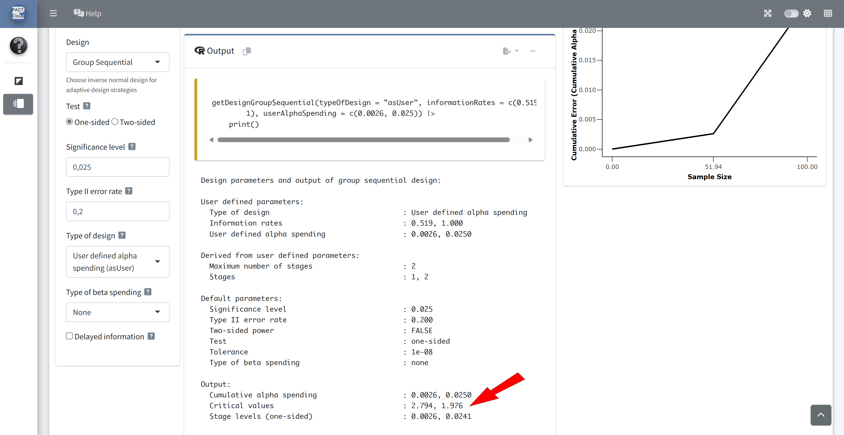
informationRates = c(67/129, 1)

Choose user defined alpha spending function

Enter how much alpha was actually spent at the interim analysis: 0.00259

Q19 What is the final analysis decision? Reject the null hypothesis since Z = -2.0 < -1.976

Note:

• The easiest way to perform boundary re-calculations is to use getAnalysisResults() with the argument maxInformation, e.g., getAnalysisResults(design, dataInput, maxInformation = 121).
• See the vignette An Example to Illustrate Boundary Re-Calculations during the Trial with rpact

More Complicated Survival Distributions

• Let’s go back to our fixed sample size design with 3.5 years of recruitment (Q4).
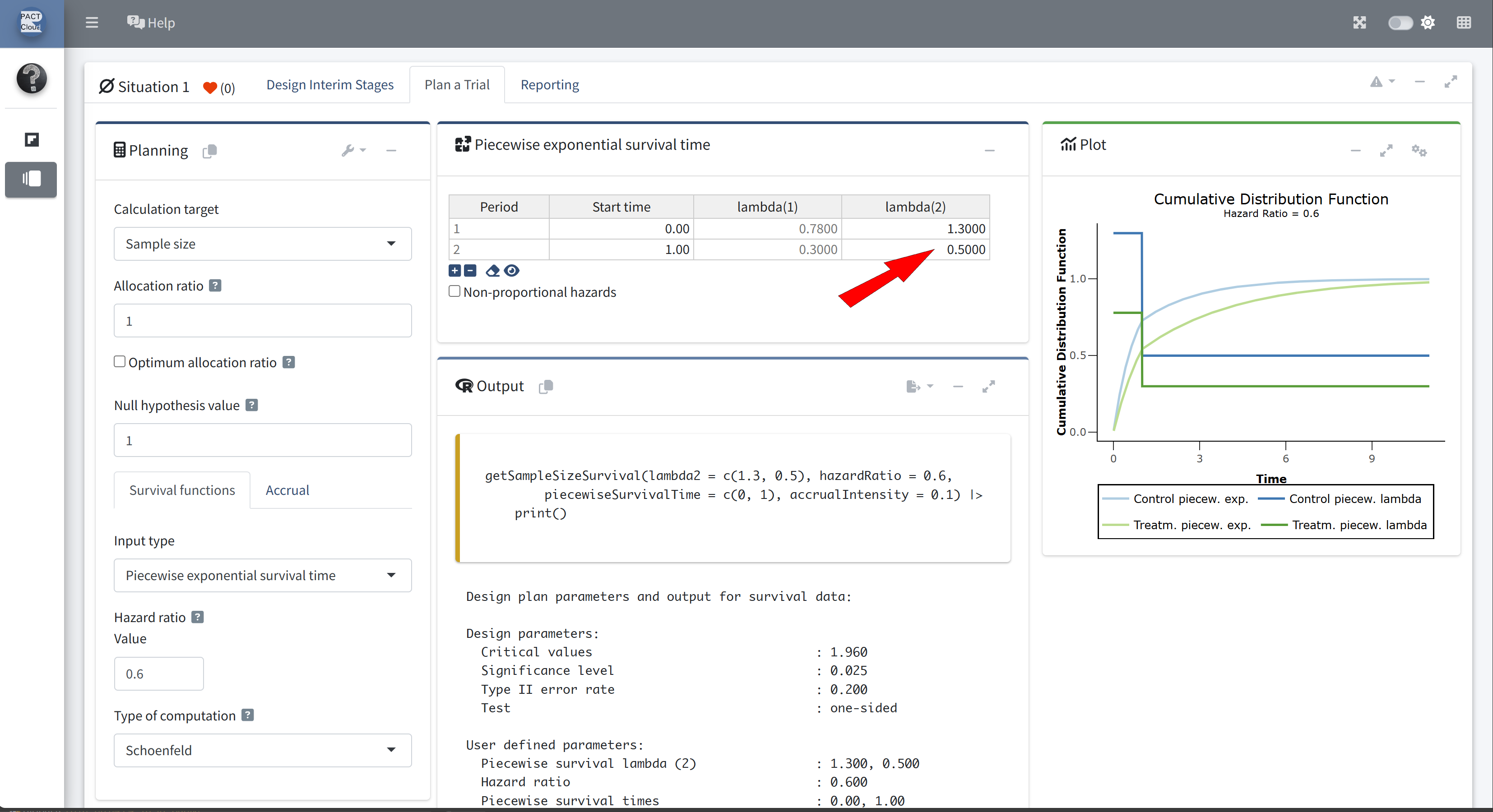
• Suppose now that the control arm follows a piecewise exponential distribution.
• For the first year the hazard rate is 1.3, and thereafter the hazard rate is 0.5.

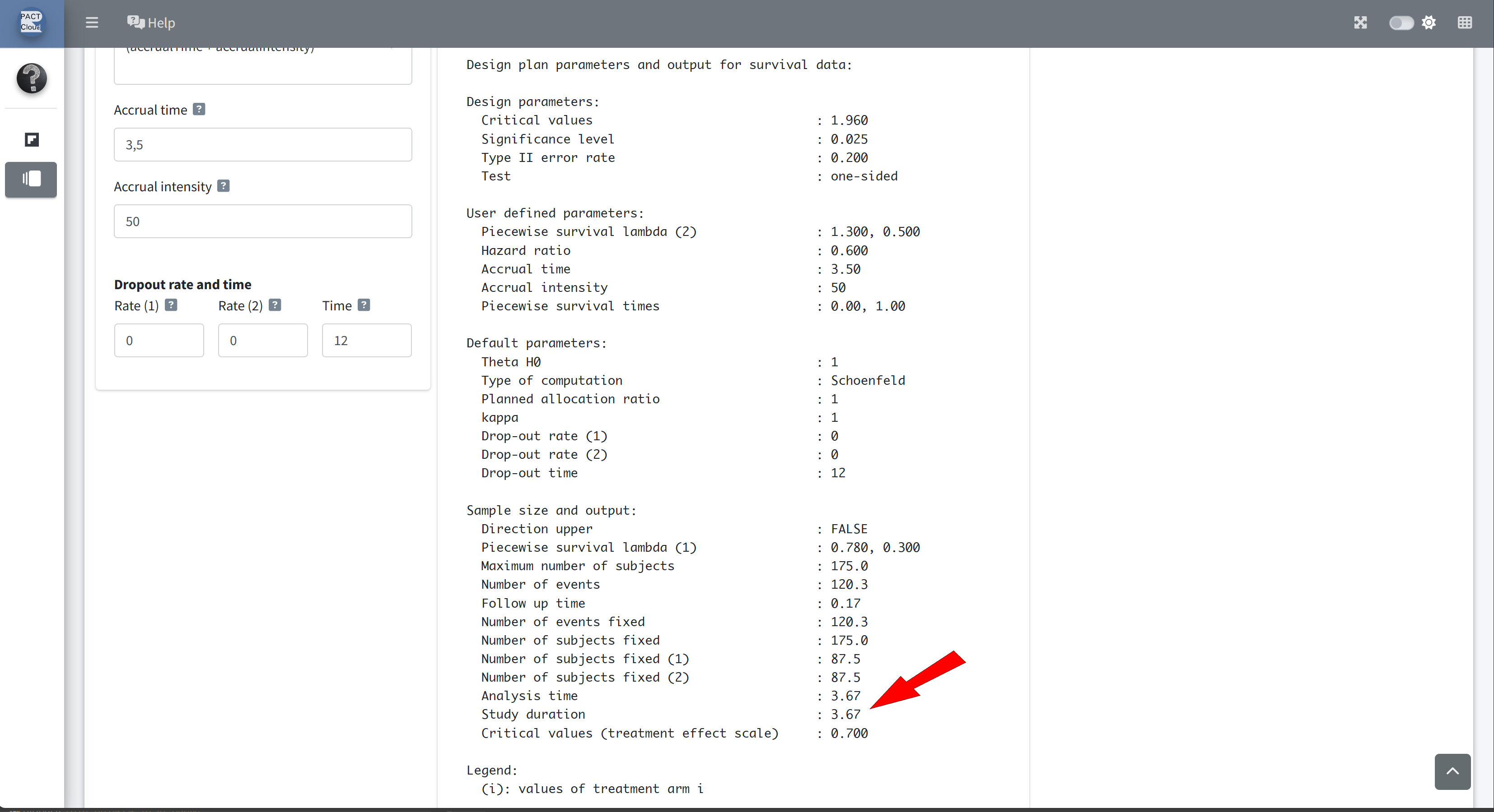
Q21 What is the expected study duration?

Choose Fixed, Survival, 2 Arms, Sample Size

Choose an appropriate survival function input type

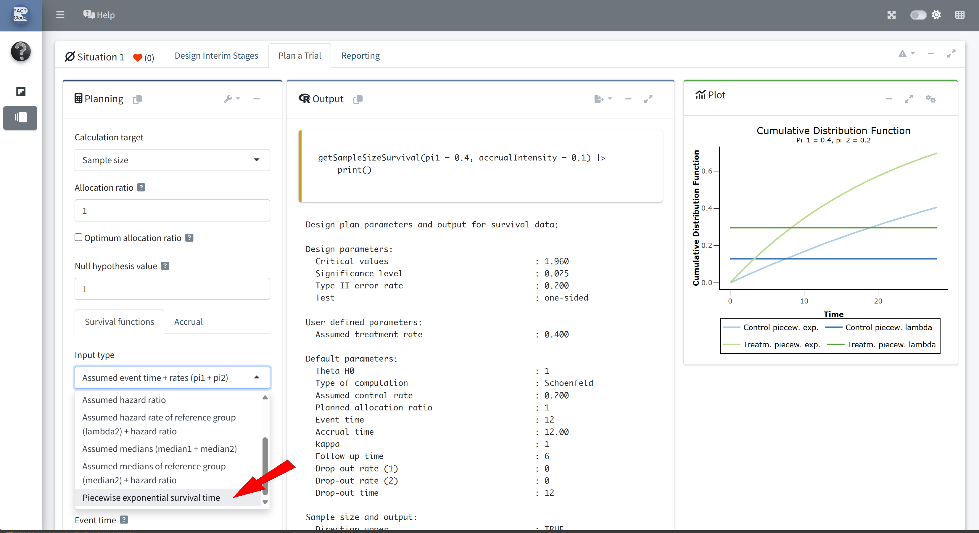
Click + to add an additional piecewise survival row

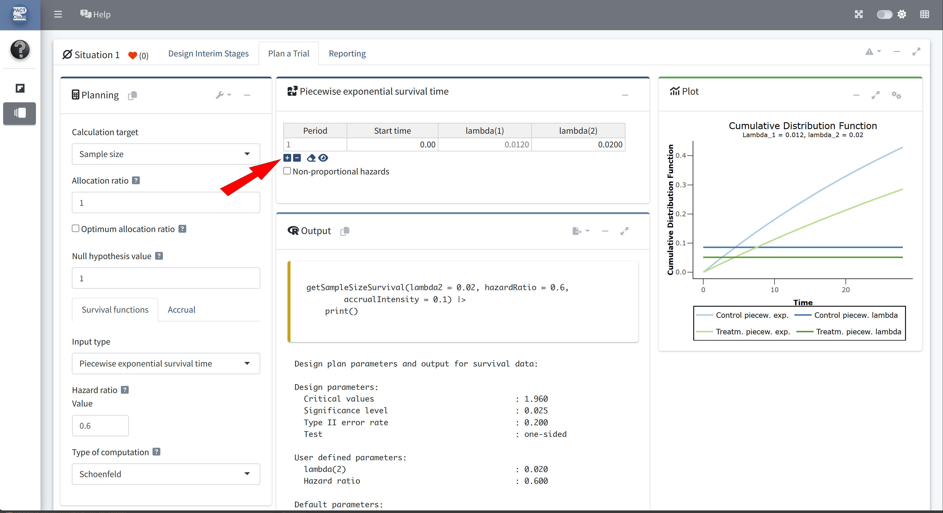
Enter appropriate start time and lambda(2)

Choose an appropriate accrual time input type

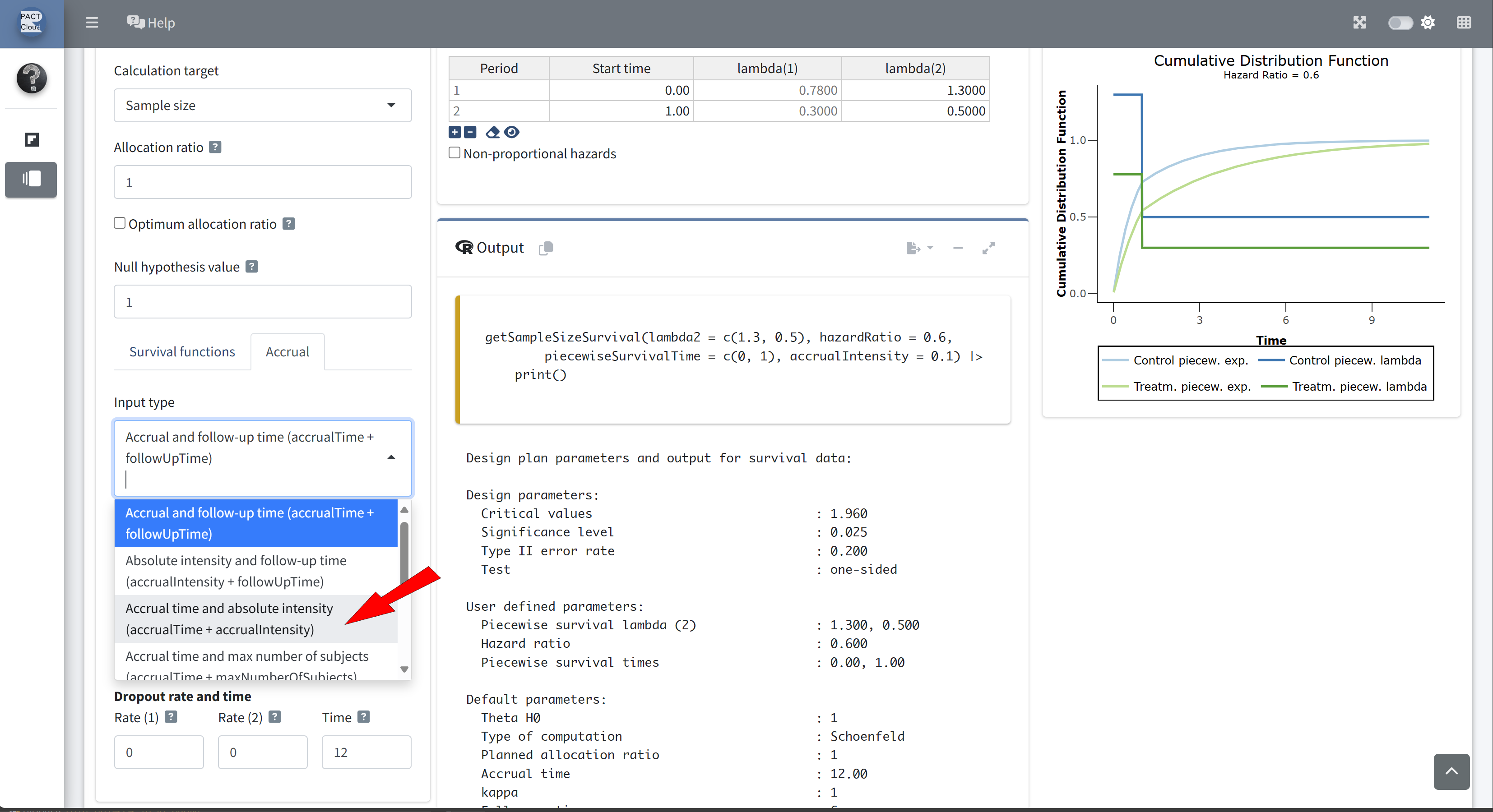
Enter accrual time 3.5 and accrual intensity 50

Q21 What is the expected study duration? \(\rightarrow\) 3.67 years

Non-proportional Hazards

• Suppose that, in addition to the changing hazard rate on the control arm, the hazard ratio also changes.
• Suppose that the hazard ratio during the first year is 0.6.
• Thereafter, the hazard ratio is 0.8.

Q22 Use the function getSimulationSurvival to calculate the power of the fixed sample size design with 3.5 years recruitment (50 subjects per year).

Choose calculation target Power simulation

Set the direction to lower (directionUpper = FALSE)

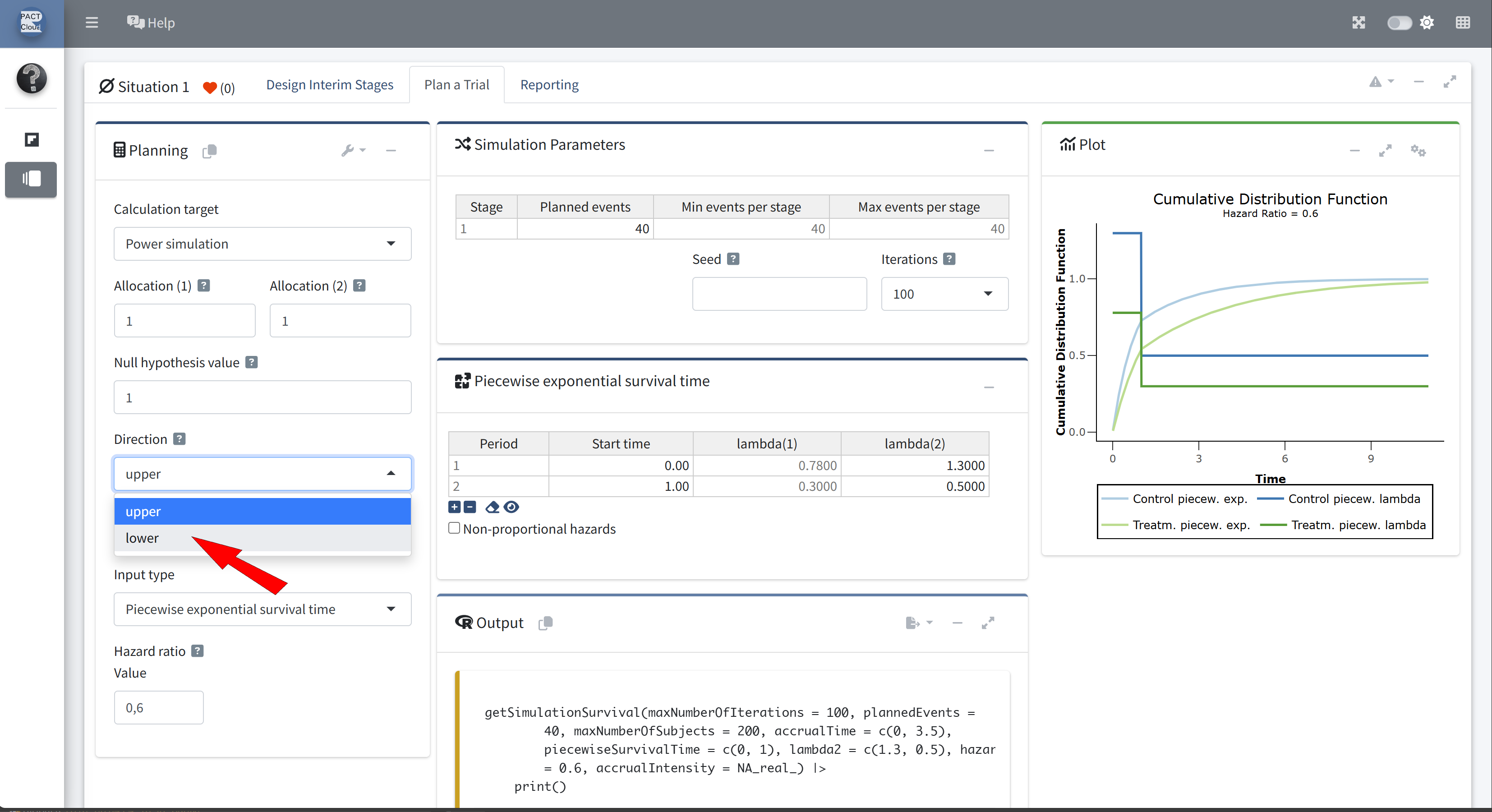
Set planned events to 121 and increase the number of iterations

Enable non-proportional hazards and set the hazard ratio to 0.8 at stage 2

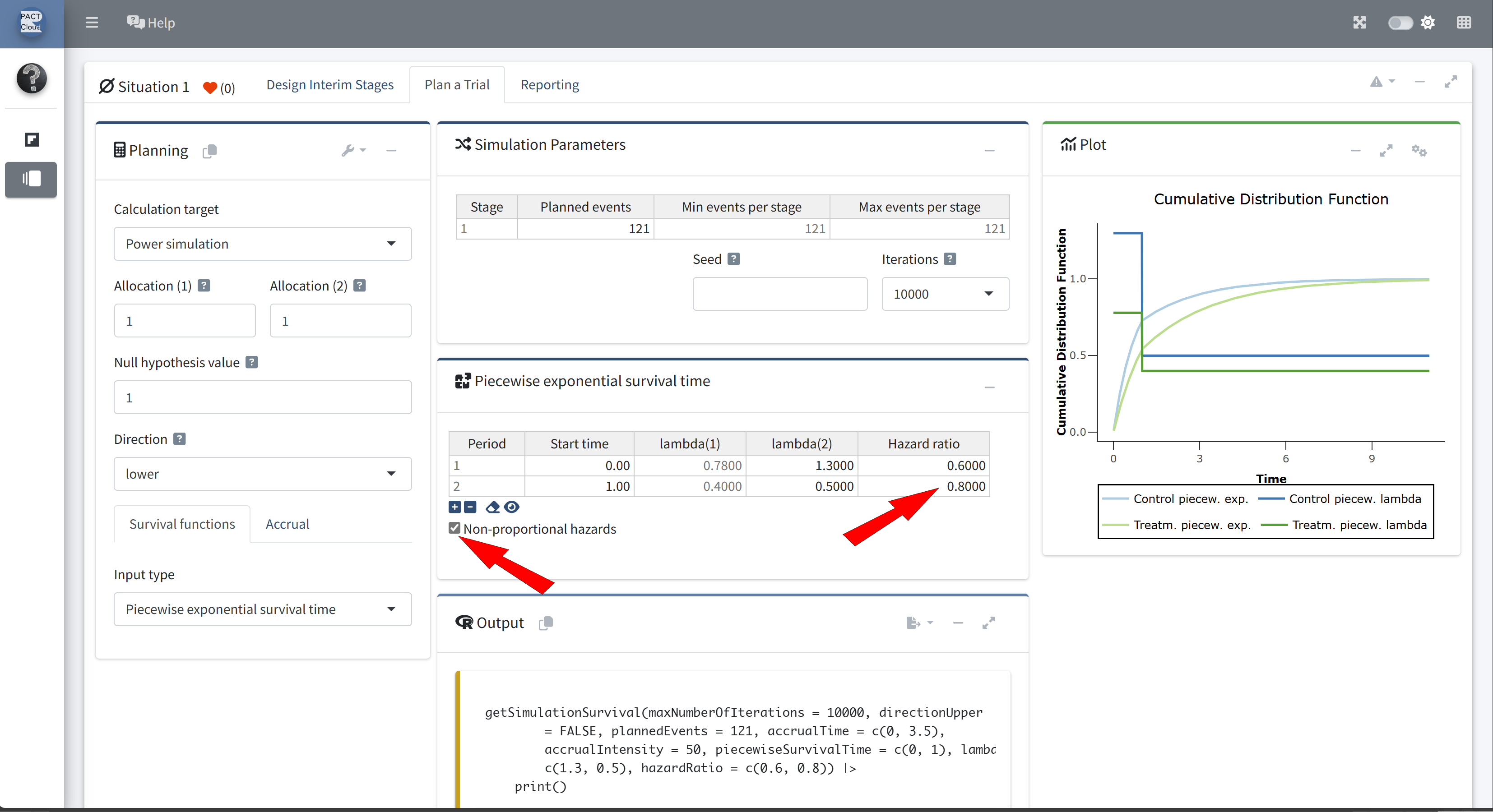
The simulated power is 0.727

Drop-outs

Drop-out assumptions can be added to any sample size or power calculation.

Q23 Going back to the assumptions in Q3, what is the expected study duration for a fixed sample size design if we specify in addition that 2% of subjects on each arm will drop out per year?

Enter dropout rate and time

Q23 What is the expected study duration?

What have we learned today?

• RPACT Cloud
  • Basic features of the GUI
  • Reporting
  • Export (qmd, Rmd, html, pdf)
  • Plotting
  • Design comparison
• Practical survival exercise

Thank you!

Questions and Answers